Lecture 1F, 08 Jan 1999
3. Trajectories of a vectorfield
Each vector is now going to be interpreted as a velocity vector. Suppose that units have been agreed for measuring both space and time, say feet and seconds, and that speeds are given by the velocity vectors accordingly in feet per second. For example, let the vector at the point p indicate a forward velocity of 15 fps.
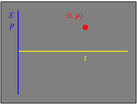
Orient the state space (blue) and the velocity vectors (green) vertically. Extend a new dimension (yellow) horizontally corresponding to time. Finally, we choose a time, t, for this construction.
| Here is the space-time plane, showing the agreed units and the chosen point, (t, p). |
|
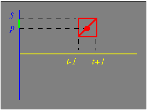
NOTE: if the vector at p had pointed down, we would have drawn this diagonal from the upper left corner to the lower right.
| Here is the direction element at the chosen point. |
|
To illustrate the process, we choose the open
interval (0, 2) as S, and the logistic function
 as the vectorfield.
| Here is a view of this vectorfield, shown in the tangent bundle representation. |
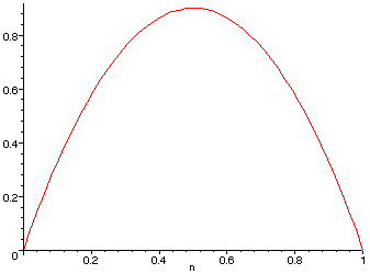
|
| And here is a plot of the direction field of this vectorfield, with trajectories superimposed. |
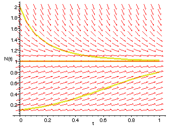
|